Analysing STA logger mapping data
Not only does the STA logger record, process and deliver your spray data automatically to an easy to view web portal, but it is also analysis ready. In this article we’re going to explore how you can analyse your weed mapping data and derive some of the advanced metrics.
Note: The analysis in this article is conducted in ArcGIS Pro (v2.8.1) which requires additional licensing. Analysis can be done in other desktop GIS applications, but the exact processes may differ.
For the analysis, we’re going to use data from three backpack units operated by an organisation called Southern Conservation Services (SCS), based in South Australia. We’ll focus on a single site called Moana Sands located near Adelaide (South Australia) where SCS conducted multiple rounds of weed control over a 6 month period in 2021.
There is a lot of data on the site which can be difficult to wade through, but hopefully by this point you are aware of the time slider tools available in the web application and ArcGIS Pro which will help you filter by time, and step through date by date.
Download and clip data
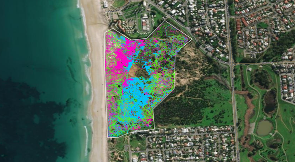
The first task we need to complete to analyse weed mapping data is to download the relevant data from the hosted web layers and separate it from the rest of the SCS data. To do this, we will use a site boundary polygon. We at TerraLab don’t know the exact boundary of the Moana Sands site but assume that in your case, you may have an existing site boundary polygon or other relevant data. So for the purposes of this analysis we’ll estimate it. When looking at the data the extent of the site becomes very obvious. We were able to create a polygon feature class and draw it based on the property boundaries and extent of STA logger data we saw.
Then we could perform a “Select by location”, ensuring to select anything that intersected with the site boundary (plus 100 metres, just to be sure). Once the selection was made, we then exported the layers to a local geodatabase (Hint: you can run the “Feature Class to Feature Class” geoprocessing tool in “batch” mode to export all layers at once. They will retain their original name if you specify the output name as %Name%).
Merge
Now the data we want to analyse is on our local machine and separated out from all of the other great data that SCS have. To perform an analysis on any of the layers, it is useful to have all feature classes combined into one. That way we can perform an analysis task once, and it summarises all work for the site. To do this, we can perform a merge on the points, tracklogs and spray zones feature classes and add “_Merge” to each name (e.g. tracklog_Merge).

Note, ensure you check the “Add source information to output” button. While the tracklog and spray zones have a field denoting the name of the device, by default, the points layer doesn’t. So by checking this button a “MERGE_SRC” field will be added and populated with the name of the device which will help you differentiate units later.
Quick stats
Now we have merged the data from different units into single feature classes, we can open the attribute table of each feature type (point, line and polygon) to get a picture of all of the data in one place. The tracklog data usually has the fewest rows so is often the easiest to review. Open the “tracklog_Merge” attribute table and sort the “GPS_Date” field in descending order. Now you will see the most recent date of work at the top, and the earliest work at the bottom. From this quick review we can see SCS first visited Moana Sands (with STA loggers) on the 9th of February 2021, and the most recent visit was the 6th of July.
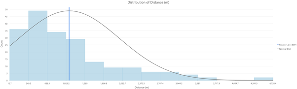
To review statistics for a given attribute, we can right click on the relevant field header and select “Statistics”. This will open a chart which we can use to quickly see that the maximum distance the operators travelled in a day is 4.7 kms, but the average is 1 km.
Detailed stats
We can plot this temporally to see all of the periods of work. Right click on the “tracklog_Merge” layer, and select “Create Chart” > “Bar Chart”. The chart properties will open. We will set the “Category or Date” to the “GPS Date” field, “Aggregation” to “Sum” and “Numeric field(s)” to “Distance (m)”. This is our result:
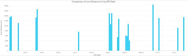
There are many more options we can configure, but this gives us a good snapshot of when they visited the site, and how far they travelled upon each visit.
Now for something far more meaningful. We can do the exact same process, but for the spray zone data. However, instead of using the “Distance (m)” field, we use the “Area (m)”:

Instead of showing the distance traversed during each visit, this graph is showing an estimate of how much area was sprayed per visit. The vertical bars look very similar to the tracklog graph because the team is constantly spraying at this site so the ratio of spraying to walking is similar. However, if you look closely, you can see that the spray zone bars between May and June (autumn in the southern hemisphere) are the tallest, sitting about 50% higher than the rest. This suggests that they were doing much more spraying during those visits indicating a potentially higher cover of their target weeds.
Reporting weed mapping stats
To this point, many of this stats may be useful for estimating resources for projects, projecting for the future, looking for efficiencies and things of that nature. But what about the key reporting criteria? If we were asked to summarise the weed levels in a simplified way, how would we do it? After all, the STA logger markets itself as a “map and treat” system in one. To do this, we will leverage off of the processes we have already investigated above.
For starters, we need to know the size of the site. The polygon we drew for the Moana Sands site is 24.09 hectares, which we can derive from the features attribute table. If it isn’t shown, you can add a new field, and use the “Calculate Geometry” process to calculate the area in whatever units and whatever projection you like.
Next, we need to segregate the spray zone data into “runs”. What we mean by that is to group the dates into discrete periods of time. For simplicity, we decided to group the data into 3 runs. That means all of the data from February and March is pooled into Run 1, April and May for Run 2 and June and July for Run 3. For each run, the data relevant to that period was exported into separate feature classes named Runs 1, 2 and 3, respectively.
We know from discussions with SCS that the ‘0’ on the selector switch was used to denote Gazania spp. (Gazanias) so we will focus only on instances where the selector was ‘0’.
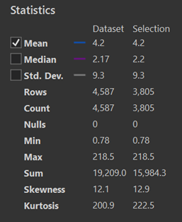
Starting with Run 1, we then made a selection (“Select by Attribute”) where the “Selector” field was ‘0’. This is a very basic SQL expression: “FIRST_SELECTOR = 0”. Then we opened the attribute table for the feature class, right clicked on the “Area” field heading and selected “Statistics”. There is a lot of valuable information there, but of critical importance is the “Sum” statistic for the Selection which is 15,984.3. This value is in metres squared (m2), so to convert that to hectares we divide by 10,000 which is 1.6 hectares.
Now, it is simple to calculate the percentage (%) area of the site that was sprayed targeting Gazanias during Run 1 by calculating:
(1.6 / 24.09 ) x 100
Area of Gazanias sprayed (ha) / Site size (ha) x 100
… Which is 6.64%. If we assume that the operators sprayed all of the Gazanias that they could find during that run, this figure can also be interpreted as the cover of the weed that was present at that time. In essence, weed cover mapping while spraying. How great is that?
Next, we repeat the process for the other two runs and determine that the cover for Run 2 was 10.0% and Run 3 was 4.3%. So with continued control of weeds over time, we are also getting snapshots of the fluctuations of the weed cover at no extra expense.
At this point it comes down to the operators and ecologists to interpret whether this fluctuation was a result of work effort, seasonal variations, or actually decreasing the cover of the weed.
Other analysis
Discussed here were some basic analysis that can be done on STA logger data. But don’t stop there! We mentioned work effort above: By analysing the first and last spray times of the point data, you can determine how many hours were worked for each spray run. Then you could also determine the average area sprayed and distance travelled of your operators per hour. How powerful would it be to have a meaningful estimate of how much area they can spray in an hour?
Furthermore, if there is analysis you need to perform routinely, you can always build it into a geoprocessing model or python script and run it whenever you require.
If there is an attribute that you want to review and the STA logger collects the data, feel free to reach out and we will give you some pointers on how to get the most from it.
Hopefully this article has given you some tips on how to analyse weed mapping data using STA logger data and GIS.
For assistance, reach out to support. For larger analytical projects, feel free to reach out to the STA logger developer, TerraLab.
Recent Posts

STA logger onboarding
Read More »
So, why the STA logger?
Read More »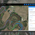
Project and herbicide reporting using the STA logger
Read More »
Why weed control contractors are flocking to use the STA logger
Read More »